A Simple Illustration of a Conceptual Soil Erosion Model

Abstract

A simple analytical solution is developed and experimentally tested for rain-impact induced erosion and sediment transport based on a recently proposed mechanistic model (Hairsine and Rose, 1991, Rose et al., 1994, Lisle et al., 1998). The model was originally derived for hillslope erosion and is reduced in this study to describe erosion from a horizontal soil surface under constant shallow overland flow (approximately 5 mm). Simulated rainfall rates were systematically changed between 15 mm hr^-1 and 100 mm hr^-1. The soil used in this study is composed of only two particle size classes, clay and sand. The model solution compares well with the experimental results (R²=0.9) and both the solution and experimental results corroborate well with the original conceptual model. This study also confirms the physical development of a heretofore-hypothesized deposition layer that eventually completely shields the underlying soil (Sander et al., 1996). Because of this study's simplicity, the physical processes are easily visualized via photographic documentation and, hence, the mathematical description readily understood; especially the development of a "shield" over the original soil and associated changes in sediment concentrations in the runoff.

Top of Document

Introduction

Though, after half a century of study, water-induced soil erosion mechanisms continue to stir controversy, it is widely recognized that upland erosion is largely initiated by the impact of raindrops on the soil surface. Recently, Hairsine and Rose (1991), Rose et al. (1994), and Lisle et al., 1998 developed a physically-based model of rain impact soil erosion on a hillslope. The conceptual model proposed by Hairsine and Rose (1991) and Rose et al. (1994) addresses the situation where the shear forces of overland flow are insignificant and surface runoff merely transports sediment entrained into the flow by the energy of falling raindrops. Lisle et al. (1998) and Rose et al. (1998) mathematically justified the model by comparing it to a generalized form of Einstein's (1937) classical stochastic model of river bedload transport. The model has been tested against a limited amount of experimental data (Proffitt et al., 1996). This study's objectives are to experimentally address some of the model's fundamental aspects not addressed by earlier experiments and, perhaps more importantly, to present the conceptual model and associated experiments in such a way that the fundamental principles are well demonstrated and easily elucidated.

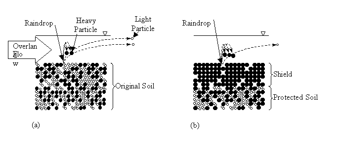
Central and unique to this model is the development of a "shield" composed of relatively heavy soil particles that protects the underlying soil from rain impact erosion. A simplified description of the process is illustrated in figure 1. When a soil surface is initially impacted with raindrops, soil particles are detached from the soil surface and entrained into the overland flow (figure 1a). Light particles, with low settling velocities, will move far from their original point of dislodgment and heavy particles will settle quickly, near their original positions. If this process continues, eventually most of the light particles will be removed leaving a shield of heavy particles that protect the underling soil (figure 1b). The full process obviously involves deposition, reattachment, and many soil-size classes or distribution functions and is fully described in published papers by Hairsine and Rose (1991), Rose et al. (1994), Sander et al. (1996), Rose et al. (1998), and Parlange et al. (1999).

Laboratory experiments demonstrating the model's conceptual basis (Proffitt et al., 1991) have been compared to analytical/numerical solutions of the model by Sander et al. (1996), Hogarth et al. (1999), and Parlange et al. (1999). These studies, using Proffitt's et al.'s (1991) data, have shown strong agreement between model results and experimental data. However, the experiments were, in many ways, too complicated to elucidate the fundamental conceptual model; e.g. the roles of interdependent parameters were difficult to ascertain from the experiments alone. The primary purpose of this study is to explore the erosion concept proposed by Haisine and Rose (1991) and Rose (1994) via as uncomplicated an experiment as possible. One objective of this study is to definitively document the formation and protective nature of the surface shield; this was not explicitly observed or measured in the Profitt et al. (1991) experiments, though it was strongly implied by the temporal decrease of sediment concentration in the overland flow. Several of the studies mentioned above have suggested the theoretical existence of a complete shield, which virtually prohibits further erosion. Such a shield would only develop on a flat soil surface; i.e. a surface on which the entrained particles would experience no persistent, unidirectional migration. On sloped surfaces the entrained particles continuously jump downslope thus the shield continuously drifts leaving the upslope subsoil partially unprotected. The experimental set-up in this study employs a horizontal surface that facilitates investigating the development of complete shielding.

Top of Document

Model Derivation and Parameterization

This study investigates the simple situation in which there are only two soil classes, clay, which, once entrained into the flow, never settles and sand which settles very rapidly. Other simplifications include constant depth and no spatial dependencies. Following the definitions of Sander et al. (1996), each particle class contains the same mass of original soil material. Consider a soil composed of 9 parts sand to 1 part clay by mass. To apply the model to this medium, the soil is divided into 10 classes one class of clay and nine identical classes of sand:

(1)

The different classes are characterized by their concentrations in the suspension, c [M L^-3] and by their masses per unit area in the deposited layer, M_d [M]. The settling velocity of the clay particles is slow, and within a limited time scale, is negligible, i.e. essentially zero. In contrast, the sand particles settle very quickly and are primarily found in the deposited layer.

(2)

For this simple scenario, equation (9) of Sander et al. (1996) can be written for the clay fraction as:

(3)

Where c₁ is the concentration of clay in the surface flow [ML^-3], D is the flow depth [L], P is the rainfall rate [LT^-1], and I is the number of particle size classes characterizing the soil (i.e. I=10); each class represents an equal mass fraction. The term Pc₁, is the mass flow rate of clay particles out of the system. The parameter a is the bare soil's detachability [ML^-3] and b is another soil parameter (dimensionless). H represents the shielding state of the soil. A shielding state, H=0, corresponds to no shield and H=1 to complete shielding and full protection from further erosion. The original model addresses the additional process of redetachment of deposited material; the scenario investigated here doesn't involve this process because the heavy particles instantly settle. In the scenario described here, the hypothesis is that the clay erodes away and a sand deposition layer accumulates to shield the underlying soil

The total mass of sand in the deposited or shield layer is. Following Sander et al. (1996) the conservation of mass for the sand fraction is:

(4)

The shield, H, as defined by Sander et al. (1996) is expressed as:

(5)

Where is the total mass of the deposited material (sand) in the shield once it is complete.

Equation (4) can be solved using the initial condition M_dt=0 at t=0 to yield:

(6)

Substituting (6) into (5), the formation of the shield, H, is:

(7)

The parameter can be replaced by the total mass of eroded particles, 9, since the ratio of masses in the original soil is known; i.e. . The mass of clay removed from the original soil, M₁*, can be calculated by integrating the product of measured clay concentration in the suspension (c₁) and the flux, which for our steady state experiments is the rain rate, P:

(8)

Inserting the expression for H in equation (7) into equation (3) yields a linear first order equation for which, using the initial condition c₁=0 at t=0, the solution is:

(9)

Comparison among experiments can be streamlined via normalized, dimensionless parameters. Consider the following dimensionless variables:

, , and (10)

From the definitions in (10), a simple relationship between the dimensionless concentration variable, C, and the dimensionless time variable, T:

(11)

Because each experimental run has a unique l , equation (11) gives unique curves for each run. Rewriting equation (11) in the following form will ameliorate this uniqueness and allow simple verification of the quality of agreement between the model and data:

(12)

The term on the left-hand-side of equation (12) is referred to as the transformed concentration, Ct .

Top of Document

Experimental Methods

The laboratory experiments are designed to be as simple as possible and for this study the only controlled variable is rainfall rate; all other parameters are kept as constant as possible. The experimental set-up is schematically diagramed in figure 2. A small, Plexiglas cube (7x7x7 cm) is filled with an artificial soil and leveled 2.1 meters below a rainmaker. After carefully establishing an initial pond depth of 5 cm on the soil, rain is simulated over the box and an overflow spout in the side of the box maintains constant ponding depth (Figure 2). Five experiments are run at different rain rates (15 - 100 mmh^-1). Outflow is periodically collected from the overflow spout with an automatic fraction sampler. In the first stage of each experiment, samples are collected every 15 to 30 seconds (depending on the rainfall rate), later, samples are collected at longer intervals. Each experiment continues until the ponded water is completely clear, 1.5 to 5 hours depending on the rainfall rate. The sediment concentration of each sample is measured using a spectrophotometer (Bausch & Lomb, Spectronic 1001, 546.1 nM wave length). In these experiments, water is always distilled.

The soil, 90% sand (180m - 212m) and 10% clay (hydrous Kaolin supplied by Englehard Corp, NJ), is prepared as a saturated mixture in order to minimize clay aggregation. The soil is put into the Plexiglas cube and allowed to settle. The surface is smoothed and leveled under the rainmaker. Pre-ponding is achieved by placing a strip of paper on the soil surface to prevent erosion during the pre-ponding process. Water is carefully pipetted onto the paper until to achieve an appropriate ponding depth after which the paper is removed with minimal disturbance to the soil. The rainmaker is then turned on and a timer started simultaneously.

Rainfall is simulated using a 20 cm diameter, water-filled Marriotte cylinder rotating at about 20 rpm. The bottom end of the cylinder is pierced by hypodermic needles (B-Dâ 21g1.5). The rainmaker is placed near the ceiling of the Soil and Water Laboratory at Cornell University's Agricultural and Biological Engineering Department, 2.1 meters above the soil-cube. Rain rate is increased or decreased by adding or removing needles respectively. Needle distribution is determined by trial and error until a uniformity of 85% or greater is achieved. Uniformity is determined using nine vials (1.5 cm diameter) evenly distributed over the soil-cube position which catch 30 minutes of rain; after determining the standard deviation and average for the nine catches, uniformity=1-(standard deviation)/(average). The rain simulator produces drops of ~1.7 mm radius. Ignoring air resistance, the energy per drop is approximately 4312 ergs and the total energy per 1 mm of rain is 19.6 J m^-2. This is similar to energy from the Proffitt et al. (1991) experiments, 22.8 J m^-2 per 1 mm of rain, which simulated rain from 9 m above the soil surface.

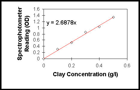
Upon completion of each experimental run, the samples are diluted to fit into the range of the spectrophotometer calibration curve made prior to the experiment. The calibration curve, shown in figure 3, is developed by correlating a set of solutions of known clay concentration to respective optical density (OD) readings; for these experiments OD = 2.6878[clay]. The calibration curve has an R² value of 0.995 and an error of less than 4%.

Top of Document

Results and Discussion

To determine the unknown soil constants, a and b, the l's are determined to best-fit the two experimental runs that represented the extreme rain intensities, P=15 mm hr^-1 (run 1) and P=100 mm hr^-1 (run 5). The soil constants are determined from these two l's by using the expression for l in equations (10). The soil detachability, a, is 437 mg cm^-3 and the b parameter is 1.05. These values for a and b are used to model the other experiments. The depth, D, is 0.5 cm for all runs. The other parameters and model-agreement statistics for each of the five experimental runs are shown in table 1. The total mass of eroded material, M₁* is determined by integrating the data over time. The R² are consistently near 0.9 indicating good general correlation between predicted and observed sediment concentrations, c. The relative difference is consistently near 20%. Good agreement between model results and observations is seen in figure 4 which shows Ct for all the runs (R²=0.96).

The detachability of a Solonchack soil determined by Proffitt et al. (1991), ~50 mg cm^-3, was an order of magnitude lower than determined for the artificial soil used in this study. Such differences in soil parameters are expected because the composition of the soil used in this study is unique. The b exponent is often assumed to be unity (e.g. Sander et al., 1996, Hairsine et al. 1999) and this study generally supports this assumption with b very slightly greater than one; taking b=1 a priori minimally affects the agreement between the model and data. Proffitt et al. (1991) experimentally determined b slightly less than one, ~0.8-0.9.

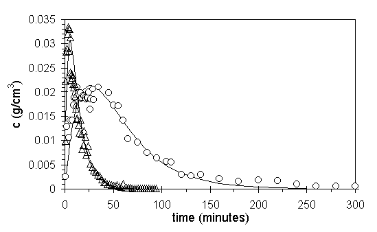
Figure 5 shows temporal trends of the raw data and associated model results for the extreme rain rates, P = 15 mm hr^-1 (run 1) and P = 100 mm hr^-1 (run 5). To avoid clutter, only two experimental runs are shown. The trends agree with the model theory. Initially, the concentration increases with time as clay is eroded from the soil and the rate of erosion decreases as the shield forms. Eventually the shield protects the soil enough that the erosion rate is sufficiently slowed such that the temporal trend in concentration is reversed; the concentration of clay in suspension decreases because more clay is leaving in the overland flow than is being eroded from the soil. In our special case of a level soil surface, the shielding approaches completeness; this claim is corroborated by the fact that the clay concentrations go to approximately zero for long times. As expected, the low intensity curve (circles) peaks later than the high intensity curve (triangles) because of a smaller rate of shield-building raindrops. Under "natural" conditions the time to peak may vary with raindrop size, speed, and other energy and momentum parameters but in these experiments raindrop characteristics are identical for all experiments.

The dynamic formation of the shield during an experiment is illustrated in figure 6. The shield is clearly visible as the dark layer of sand at the surface of the soil in figures 6a-6d. Notice how quickly the shield develops, it is clearly visible after 18 seconds (figure 6b). Within the first 5-10 minutes the shield is nearly complete and does not grow significantly over the next several hours. This qualitatively agrees with model solutions in previous studies especially Parlange et al. (1999). It is also obvious from the clear water in figure 6d, compared to 6b and 6c, that the shielding is complete, halting erosion. The water is also clear in 6a, before rain commences.

Top of Document

Conclusion

Using conceptually simple experiments, the rain-impact erosion model proposed by Hairsine and Rose (1991) and Rose et al. (1994) was tested and was corroborated well by the data. Because of the experimental simplicity, it was possible to reduce the model to a few simple parameters and thus illuminate the validity of basic concept. In particular, this research visually and quantitatively displays the formation of a "shield" during rain-impact erosion; this is a unique aspect of the model not widely recognized in other erosion models. These experiments also verified the heretofore-hypothesized existence of a "complete" shield that fully protects the underlying soil and justified unity for the b parameter assumed by earlier researchers. It is clear that the next step needed in this arena of research is exploration of a physical shield description (work in progress)

---

Figure 1: Schematic of soil shield development from (a) initial rain impact to (b) developing shield.

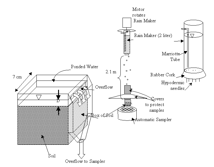
Figure 2: Schematic of experimental set-up.

Figure 3: Calibration curve for the spectropotometer: data are shown as open diamonds and the line depicts the correlation (R²=0.995).

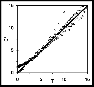
Figure 4: Comparison between observed and theoretical C^t(T); composite R² = 0.96; Each symbol is a unique experimental run (table 1): circles: run 1, diamonds: run 2, squares: run 3, solid triangles: run 4, open triangles: run 5. The line shows the model.

Figure 5: Temporal concentration changes: circles: P=15 mm hr^-1 (run 1), triangles: P=100 mm hr^-1 (run 5); lines: modeled results; see table 1 for other parameters associated with each run.

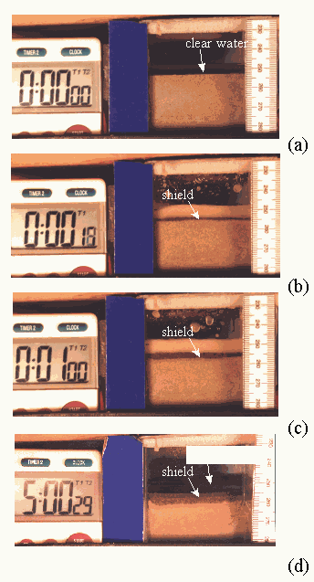
Figure 6: Photographs of shield development during an experiment.

Top of Document

References

Einstein, H. 1937. Der Geschiebebetrieb als Wahrscheinlichkeits-problem. Verlag Rascher, Zurich (Engl. Trans. In: Shen, H. (ed). 1972. Sedimentation. Symposium to honour H.A. Einstein and H.W. Shen. Fort Collins, CO).
Hogarth, W.L., Rose, C.W., ., Lisle, I., Parlange, J.-Y., Sander, G.C., Hairsine, P.B., and Cary, G. 1999. Unsteady soil erosion due to rainfall impact: Numerical solution and comparison with experimental data. J Hydrology. (in press)
Hairsine, P.B. and Rose, C.W. 1991. Rainfall detachment and deposition: sediment transport in the absence of flow-driven processes. Soil Sci. Soc. Am. J. 55(2):320-324.
Lisle, I., Rose, C.W., Hogarth, W., Harisine, P., Sander, G., and Parlange, J.-Y. 1998 Stochastic sediment transport in soil erosion. J. Hydrology. 204(1-4):217-230.
Parlange, J.-Y., Hogarth, W.L., Rose, C.W., Sander, G.C., Hairsine, P., and Lisle, I., 1999, Addendum to unsteady soil erosion model, J. Hydrology: 217:149-156
Proffitt, A.P.B., Rose, C.W., and Hairsine, P.B., 1991, Rainfall Detachment and Deposition: Experiments with Low Slopes and Significant Water Depths, Soil Sci. Soc. Am. J., 55(2):325-332.
Rose, C.W., Hogarth, W.L. Sander, G. Lisle, I. Hairsine, P. and Parlange, J.-Y. 1994. Modeling processes of soil erosion by water. Trends in Hydrology. 1:443-451.
Rose, C.W., J.-Y. Parlange, I.G. Lisle, W.L. Hogarth, P.B. Hairsine, G.C. Sander. 1998. Unsteady Soil Erosion Due to Rainfall Impact and Sediment Transport. Hydrology Days. AGU pub.18:245-258.
Sander, G.C., Hairsine, P.B., Rose, C.W., Cassidy, D., Parlange, J.-Y., Hogarth, W.L., Lisle, I.G. 1996. Unsteady soil erosion model, analytical soilutions and comparison with experimental results. J. of Hydrology. 178: 351-367.