| SiteCode | category | ecoregion | aquifer_type | Presumed_Vulnerability |
|---|---|---|---|---|
| Golf-2 | Golf | Allegheny | outwash | high |
| Golf-7 | Golf | Allegheny | outwash and alluvium | high |
| Golf-9 | Golf | Ridge & Valley | drained muck | low |
| Green-16 | Greenhouse | Coastal | lake beach? | high |
| Green-17 | Greenhouse | Allegheny | alluvium? | high |
| Green-18 | Greenhouse | Coastal | alluvium | high |
| Nur-2 | Outdoor nursery | Allegheny | outwash and alluvium | high |
| Nur-3 | Outdoor nursery | Great Lakes | drumlin | medium |
| Nur-5 | Outdoor nursery | Northeastern Highlands | alluvium | medium |
| ROW-1 | ROW | Allegheny/Lake Erie | lake beach | high |
| ROW-2 | ROW | Allegheny | outwash and alluvium | high |
| ROW-4-1 | ROW | Allegheny | outwash | high |
| ROW-4-2 | ROW | Allegheny | outwash | high |
| Sod-2 | Sod | Ridge & Valley | drained muck | low |
| Sod-3 | Sod | Great Lakes | drained muck | low |
| Turf-1 | Turf | Allegheny | outwash and alluvium | high |
| VegF-1 | Vegetable and fruit | Allegheny | lake and alluvium | high |
| VegF-4 | Vegetable and fruit | Ridge & Valley | drained muck | low |
| VegF-6 | Vegetable and fruit | Great Lakes | outwash? | high |
| Vine-1 | Vineyard | Allegheny/Great Lakes | glacial fan? | high |
| Vine-3 | Vineyard | Ridge & Valley | till and outwash | medium |
| Vine-4 | Vineyard | Allegheny/Lake Erie | lake beach | high |
This is the second page at Level 1 in a three-level web. It explains the project’s site selection and how samples are collected and analyzed.
Navigate: ◄ 1: Intro | ▲ Abstract | ► 3: Simple results
Deeper: 2.1.1 Categoricals geography | 2.2 Compounds | 2.3 Sampling and analysis.
2: Sites and Protocols (Level 1)
2.1 Approach and recruiting
The project plan specifies three types of sampling sites, categorical groundwater, long term groundwater, and lake. The sampling design, approach to address the type’s criteria, and recruiting differed by type.
As per NYSDEC’s recommended site targeting strategy, the majority of our categorical groundwater sites (around 85%) are in traditionally1 more vulnerable aquifer areas, such as soils on stream alluvium, glacial outwash, lacustrine sands, and beach deposits, all of which have greater intrinsic leaching potential than do other landscapes. Relatively mobile pesticides applied in these contexts would have a greater chance of leaching into groundwater. Conversely, about 15% of sites are presumptively (based on traditional soil physical theory) less vulnerable locations for leaching of pesticides, with overlying soils including glacial till, lacustrine clay/silt, or organic soil muckland, which are less hydraulically conductive or more retentive of contaminants.
During site selection, we avoided organic farm operations as categorical sites due to their avoidance of chemical pesticides. Conversely, our long-term site roster does include organic farms bordered by neighboring land uses where pesticides are applied and potentially transported into the cooperating site’s well water.
See the Interpretations page for discussion about how the early results challenge the presumption.
2.1.1 Categorical groundwater sites
==> Deeper: 2.1.1 Categoricals geography
The default sampling design for categorical sites is:
- two sets of samples per year from each of three locations on the property
- one “upgradient” location to detect pesticides entering the site in groundwater recharged on neighboring property
- two “downgradient” or “within” locations inside the site to detect pesticides in ground water that was recharged within the site.
Real sites may have no land upgradient, or only land without pesticide use upgradient. They may be uneven spatially in their own pesticide application, recharge and groundwater flow patterns, and feasibility of sampling. Most sites depart from the nominal count of 1+2 sampling points.
- describes the materialized categorical groundwater sites. Aquifer ratings with question marks are more uncertain than others.
(Items ROW-4-1 and ROW-4-2 represent a single railway corridor site (ROW-4) having two adjacent properties where wells are sampled. ROW-1 and ROW-2 also are sampled from adjacent properties.)
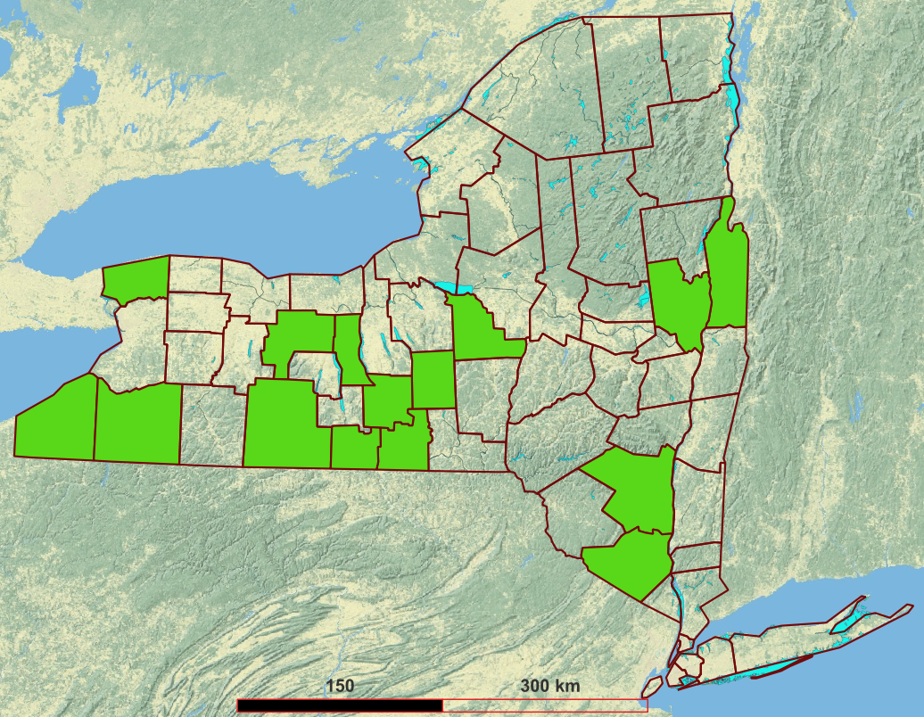
These sites (distributed as per Figure 1) were selected based on falling within one of the eight land use categories prioritized by NYS DEC for the current MOU. 1 tallies the categorical sites according to three diversity criteria besides their category.
| Attribute | Value | Count |
|---|---|---|
| Presumed leaching vulnerability | ||
| High | 9 | |
| Medium and mixed | 7 | |
| Low | 5 | |
| Soil and shallow aquifer composition | ||
| Sand and gravel (glacial outwash, kame or alluvium) | 15 | |
| Drained muck | 4 | |
| Gravel/silt loam | 1 | |
| Mixed glacial till, gravel and clay | 1 | |
| Ecoregion | ||
| Allegheny Plateau | 8 | |
| Great Lakes Lowland | 6 | |
| Ridge and Valley | 4 | |
| Coastal (Hudson) | 2 | |
| Northeast Highlands | 1 |
We classify the sampling points on categorical sites according to the position of the point relative to the cooperator’s use of pesticides. The sampling point can be upgradient (generally uphill2) from the cooperator’s pesticide use, meaning that if anything is detected it is most likely from a neighbor; the point can be downgradient (generally downhill) some distance from the owner’s pesticide uses; or the point can be within one of the owner’s pesticide use areas; within would include land a few feet downgradient but never land that is upgradient. Classifying in this way allows a more accurate connection of results to the cooperator’s own pesticide use, and also helps with sampling timing. Wells that are within a pesticide use area may have the most transient concentrations, highest shortly after leaching events soon after application, but low most of the time. Downgradient and upgradient positions involve some distance for groundwater to flow laterally after vertical groundwater recharge, thus provide opportunity for mixing of groundwater recharge from different recharge events and different parts of the property of the pesticide user.
In the majority of categorical sites, no upgradient sampling points were necessary because there was no neighbors’ land upgradient from the cooperator’s pesticide use zones.
2.1.2 Long term groundwater sites
We initially hoped to fill the long-term site roster by re-recruiting participants in earlier projects (six counties). For various reasons (including many changes of ownership in the decade(s) since the initial sampling), the needed number of sites was not reached. Following NYS DEC’s encouragement, we geographically diversified our site coverage of the state (including adding areas with no categorical sites present). In the summer of 2023, we also switched to primarily recruiting small businesses or other establishments (in place of typically non-responsive households), approaching sites ranging from arboretums to legal cannabis farms (where pesticide use can be heavy). We also went beyond the initial target of 24 sites, noting that some of the recruited sites may be provisional and not be continued past the first year or two. The roster as of the end of 2023 is shown in Table 3 . Ecoregions represented include all those for categorical sites plus some sites in the Erie Drift ecoregion.
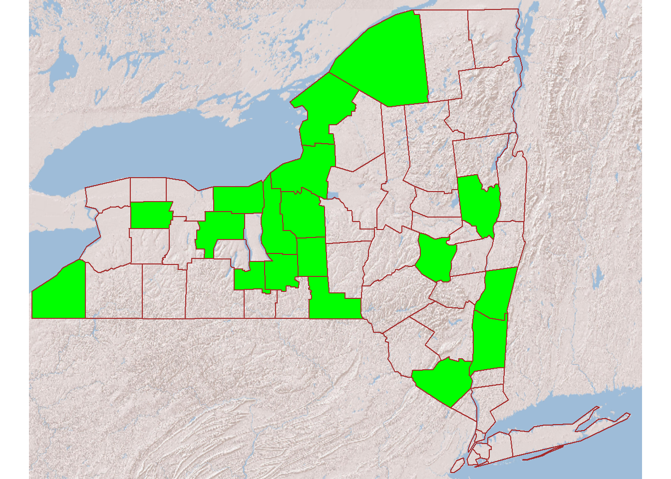
As of August 2024, this type of site drew from 18 counties (Figure 2).
.
| County | Ecoregion | Aquifer | Vulnerability | Rejoining |
|---|---|---|---|---|
| Tompkins | Allegheny | glacial outwash | high | no |
| Cortland | Allegheny | glacial outwash | high | yes |
| Cortland | Allegheny | outwash gravel? | high | yes |
| Steuben | Allegheny | outwash | high | no |
| Cortland | Allegheny | glacial till | low | no |
| Broome | Allegheny | glacial kame or till | medium | no |
| Columbia | Coastal | glacial outwash | high | no |
| Saratoga | Coastal | bedrock | low | no |
| Chautauqua | Erie Drift | alluvium | high | no |
| Chautauqua | Erie Drift | alluvium and till | medium | no |
| Jefferson | Great Lakes | lake sand | high | no |
| Onondaga | Great Lakes | glacial outwash | high | no |
| Genesee | Great Lakes | karst | high | yes |
| Jefferson | Great Lakes | lake silt/clay | low | no |
| Jefferson | Great Lakes | lake silt/clay | low | no |
| Jefferson | Great Lakes | glacial till/moraine | low | no |
| Jefferson | Great Lakes | lake silt/clay | low | no |
| Jefferson | Great Lakes | lake silt/clay | low | no |
| Onondaga | Great Lakes | glacial till | low | no |
| Cayuga | Great Lakes | till, lake silt/clay | low | yes |
| Cayuga | Great Lakes | glacial till | low | yes |
| Jefferson | Great Lakes | lake silt/clay | low | no |
| Jefferson | Great Lakes | lake silt/clay | low | no |
| Schoharie | Great Lakes | glacial till | low | no |
| Onondaga | Great Lakes | glacial till | low | no |
| Ontario | Great Lakes | perched | low | no |
| Cayuga | Great Lakes | lake silt/clay | low | yes |
| Genesee | Great Lakes | glacial till | low | no |
| Wayne | Great Lakes | glacial till, muck | low | no |
| Genesee | Great Lakes | glacial till | low | yes |
| St. Lawrence | Great Lakes | alluvium | medium | no |
| Cayuga | Great Lakes | till | medium | no |
| Dutchess | Northeastern Highlands | alluvial fan | high | no |
| Orange | Ridge & Valley | lake silt/clay | low | yes |
| Orange | Ridge & Valley | kame? | medium | no |
2.1.3 Lake sites
The contract specified four lakes sampled once per year at two sampling points each. We varied from this to reflect conditions at the actual lakes chosen and the perspectives of volunteers at two lakes. Since no four lakes could represent the hundreds of greatly varied lakes in Upstate New York, we simply tried to be diverse, spanning geography, from almost Lake Erie to almost the Connecticut border, four ecoregions, and sizes from 0.2 to 21 square miles.
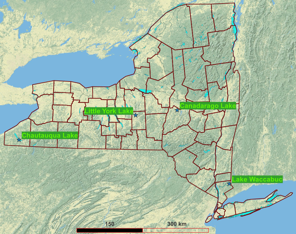
CSLAP considers the deepest point of a lake to be most representative. That and the contract recommendation of inlets and outlet conditioned where we sample lakes.
| Lake | Sampling locations | When | Samplers |
|---|---|---|---|
| Upper Little York Lake | - 2-3 near inlets, - One at outlet, - One in middle near categorical pesticide source. Significant groundwater input, lake within a principal aquifer. |
Once, spring or summer | Cornell |
| Lake Waccabuc | Standard CSLAP location; major tributary input area | Twice, late spring to early fall | CSLAP volunteers |
| Chautauqua Lake | (see text) | Once, Spring or Summer | CSLAP volunteers (2022) Cornell (2023-2024) |
| Canadarago Lake | Bridges over two major inlets and outlet | Once, Summer or Fall | Cornell |
2.2 Analyte selection
==> Level 2 detail about analyte selection
There are many, many pesticide products registered for use in New York. These contain a variety of active ingredients. For environmental fate assessment we are interested in the active ingredients, not so much the products or purposes for which they are used. A key question is, which active ingredients should be measured in groundwater and lake water? Testing is expensive and NYSDEC analytical lab time should be used most productively.
We include the most popular and slant toward active ingredients with properties that have in the past favored chemicals reaching groundwater. We also include breakdown products of selected herbicides.
Table 5 below contains the 2022-2023 list with columns for the minimum and maximum lowest analytical detection limits (DL) in micrograms per liter, a soil degradation half life in days (t_{1/2}), a sorption parameter K_{oc} or K_{foc}3, and a groundwater ubiquity score (GUS)4 that is higher when a chemical is more persisting or less sorbing. The latter column combines the half life and sorption parameter into an index that is higher when a chemical is more likely to move and persist until it reached groundwater, lower when it is less likely to move and persist.
An asterisk in a detection limit value indicates that the lab has reported values below this number, flagging the compound as present but not quantified. We abbreviate these cases as “NQD” for “Non Quantified Detections”.
| parameter | pgroup | minDL | maxDL | soil_halflife | kocORkfoc | GUS |
|---|---|---|---|---|---|---|
| 2,4-D | pesticides | <0.2 | <0.5 | 28.80 | 39.30 | 3.82 |
| Acetamiprid | pesticides | <0.01 | <0.100 | 3.00 | 200.00 | 0.94 |
| Acetochlor | pesticides | <0.25 | <0.25 | 12.10 | 156.00 | 1.67 |
| Atrazine | pesticides | <*0.01 | <0.01 | 29.00 | 100.00 | 2.57 |
| Azoxystrobin | pesticides | <0.025 | <0.025 | 180.70 | 589.00 | 3.1 |
| Bentazon | pesticides | <0.5 | <0.5 | 7.50 | 55.30 | 1.95 |
| Boscalid | pesticides | <0.025 | <0.025 | 254.00 | 772.00 | 2.68 |
| Bromacil | pesticides | <*0.05 | <0.05 | 60.00 | 32.00 | 3.44 |
| Carbaryl | pesticides | <*0.05 | <0.05 | 16.00 | 300.00 | 2.02 |
| Chlorantraniliprole | pesticides | <0.5 | <0.5 | 204.00 | 362.00 | 3.51 |
| Chlorpyrifos | pesticides | <0.025 | <0.025 | 27.60 | 5509.00 | 0.58 |
| Chlorsulfuron | pesticides | <0.01 | <0.01 | 36.20 | 36.30 | 3.80 |
| Clethodim | pesticides | <0.05 | <0.05 | 3.00 | 22.70 | 1.26 |
| Clopyralid | pesticides | <0.2 | <0.5 | 11.00 | 5.00 | 3.44 |
| Cloransulam-Methyl | pesticides | <0.05 | <0.1 | 10.00 | 30.00 | 2.53 |
| Clothianidin | pesticides | <0.05 | <0.100 | 121.20 | 123.00 | 3.74 |
| Cyantraniliprole | pesticides | <1.0 | <1.0 | 32.40 | 241.00 | 2.59 |
| Cyprodynil | pesticides | <0.025 | <0.05 | 45.00 | 2277.00 | 1.06 |
| Diazinon | pesticides | <0.01 | <0.01 | 18.40 | 609.00 | 1.51 |
| Dicamba | pesticides | <0.2 | <0.5 | 3.90 | 5.28 | 1.94 |
| Dichlobenil | pesticides | <10 | <10 | 5.40 | 257.00 | 1.19 |
| Dichlorvos | pesticides | <2.5 | <2.5 | 2.00 | 50.00 | 0.69 |
| Difenconazole | pesticides | <0.05 | <0.5 | 91.80 | 3760.00 | 0.83 |
| Dimethoate | pesticides | <0.01 | <0.01 | 7.20 | 28.40 | 2.18 |
| Dinotefuran | pesticides | <0.05 | <0.100 | 75.00 | 26.00 | 4.85 |
| Dithiopyr | pesticides | <0.01 | <0.01 | 39.00 | 801.00 | 1.74 |
| Diuron | pesticides | <0.01 | <0.01 | 229.00 | 680.00 | 2.65 |
| Endothall | pesticides | <2.5 | <2.5 | 7.00 | 85.00 | 1.75 |
| Ethofumesate | pesticides | <0.025 | <0.05 | 37.80 | 118.00 | 3.04 |
| Florpyrauxifen Benzyl | pesticides | <0.05 | <0.10 | 150.00 | 32308.00 | -0.76 |
| Fluazafop-p-butyl | pesticides | <0.25 | <0.25 | 8.20 | 3394.00 | 0.43 |
| Fluazinam | pesticides | <0.1 | <0.10 | 25.90 | 16430.00 | 1 |
| Flumioxazin | pesticides | <0.05 | <0.25 | 17.60 | 889.00 | 1.31 |
| Fluopicolide | pesticides | <0.01 | <0.01 | 138.80 | 321.10 | 3.2 |
| Fluopyram | pesticides | <0.025 | <0.025 | 118.80 | 278.90 | 3.23 |
| Fluoxastrobin | pesticides | <0.025 | <0.025 | 52.60 | 848.00 | 1.84 |
| Flutolanil | pesticides | <0.01 | <0.01 | 105.00 | 735.00 | 2.29 |
| Fluxapyroxad | pesticides | <0.25 | <1.0 | 181.50 | 728.00 | 2.57 |
| Fomesafen | pesticides | <0.5 | <0.5 | 86.00 | 50.00 | 4.45 |
| Glyphosate | pesticides | <1.0 | <1.0 | 6.45 | 1424.00 | 0.21 |
| Halosulfuron-methyl | pesticides | <0.025 | <0.025 | 14.00 | 109.00 | 2.80 |
| Hexazinone | pesticides | <0.01 | <0.01 | 105.00 | 54.00 | 4.43 |
| Imidacloprid | pesticides | <0.025 | <0.05 | 174.00 | 225.00 | 3.69 |
| Indaziflam | pesticides | <0.025 | <0.025 | 150.00 | 1000.00 | 2.18 |
| Iprodione | pesticides | <0.5 | <0.5 | 11.70 | 700.00 | 0.43 |
| Linuron | pesticides | <0.25 | <0.5 | 48.00 | 842.80 | 2.49 |
| MCPA | pesticides | <0.2 | <0.5 | 25.00 | 73.88 | 2.31 |
| MCPP | pesticides | <0.2 | <0.5 | 21.00 | 59.80 | 2.94 |
| Malathion | pesticides | <0.01 | <0.01 | 1.00 | 1800.00 | 0 |
| Mandipropamid | pesticides | <0.025 | <0.025 | 13.60 | 847.00 | 1.22 |
| Mefentrifluconazole | pesticides | <0.025 | <0.05 | 200.00 | 3456.00 | 1.06 |
| Mesotrione | pesticides | <0.5 | <0.5 | 5.00 | 122.00 | 1.45 |
| Metalaxyl | pesticides | <0.05 | <0.05 | 14.10 | 162.00 | 2.06 |
| Methiocarb | pesticides | <0.025 | <0.025 | 35.00 | 660.00 | 1.82 |
| Methomyl | pesticides | <0.1 | <0.1 | 7.00 | 72.00 | 2.19 |
| Metolachlor | pesticides | <0.025 | <0.025 | 21.00 | 120.00 | 2.36 |
| Metribuzin | pesticides | <0.025 | <0.025 | 19.00 | 48.30 | 2.96 |
| Metsulfuron Methyl | pesticides | <0.025 | <0.025 | 13.30 | 12.00 | 3.85 |
| Myclobutanil | pesticides | <0.025 | <0.025 | 35.00 | 517.00 | 1.99 |
| Napropamide | pesticides | <0.01 | <0.01 | 72.00 | 839.00 | 1.96 |
| Nicosulfuron | pesticides | <0.05 | <0.05 | 13.50 | 30.00 | 3.44 |
| Oxadiazon | pesticides | <0.025 | <0.1 | 165.00 | 3200.00 | 1.97 |
| Oxamyl | pesticides | <0.5 | <0.5 | 6.00 | 14.91 | 2.23 |
| Paclobutrazol | pesticides | <0.025 | <0.025 | 29.50 | 400.00 | 2.47 |
| Prometon | pesticides | <0.05 | <0.05 | 500.00 | 43.20 | 6.31 |
| Propamocarb HCL | pesticides | <0.01 | <0.01 | 20.00 | 706.00 | 1.5 |
| Propiconazole | pesticides | <0.01 | <0.01 | 35.20 | 1086.00 | 1.58 |
| Propoxur | pesticides | <0.05 | <0.05 | 28.00 | 30.00 | 3.65 |
| Pyrimethanil | pesticides | <0.025 | <0.025 | 31.40 | 355.70 | 2.17 |
| Quinclorac | pesticides | <0.05 | <0.05 | 450.00 | 50.00 | 6.29 |
| S-Metolachlor | pesticides | <0.025 | <0.05 | 23.17 | 120.00 | 2.32 |
| Simazine | pesticides | <0.01 | <0.01 | 90.00 | 130.00 | 2.20 |
| Sulfentrazone | pesticides | <0.25 | <0.25 | 541.00 | 43.00 | 6.16 |
| Tebuconazole | pesticides | <0.025 | <0.025 | 47.10 | 769.00 | 1.86 |
| Tebuthiuron | pesticides | <0.025 | <0.025 | 400.00 | 80.00 | 5.36 |
| Terbacil | pesticides | <*0.5 | <0.5 | 115.00 | 55.00 | 4.70 |
| Thiamethoxam | pesticides | <*0.025 | <0.100 | 39.00 | 56.20 | 3.58 |
| Thifensulfuron Methyl | pesticides | <0.025 | <0.025 | 10.00 | 28.30 | 3.05 |
| Thiodicarb | pesticides | <0.025 | <0.025 | 18.00 | 418.00 | 1.73 |
| Triadimefon | pesticides | <0.025 | <0.025 | 26.00 | 300.00 | 1.59 |
| AMPA | metabolites | <1.0 | <1.0 | 419.00 | 2002.00 | 0.04 |
| Acetochlor ESA | metabolites | <*0.05 | <0.05 | 90.00 | 28.80 | 3.73 |
| Acetochlor OA | metabolites | <*0.05 | <0.05 | 12.00 | 24.30 | 2.49 |
| De Ethyl Atrazine | metabolites | <*0.05 | <0.25 | 45.00 | 110.00 | 3.24 |
| De Isopropyl Atrazine | metabolites | <0.25 | <0.25 | - | 130.00 | - |
| Hydroxy Atrazine | metabolites | <*0.05 | <0.25 | 164.00 | - | - |
| JSE76 | metabolites | <0.05 | <0.05 | 109.00 | 30.00 | 5.23 |
| Metolachlor ESA | metabolites | <*0.05 | <0.15 | 400.00 | 9.00 | 7.22 |
| Metolachlor OA | metabolites | <*0.05 | <0.1 | 325.00 | 17.00 | 6.88 |
Explanations of columns in previous table:
| Header | Meaning |
|---|---|
| Parameter | Name of active ingredient or metabolite as used by NYSDEC lab |
| pgroup | ‘Pesticides’ or ‘Metabolites’ |
| minDl, MaxDL | Lowest and highest analytical detection limits from lab |
| soil_halflife | Degradation half life in soil |
| kocORkfoc | K_{oc} value when available, K_{foc} when K_{oc} not available, or blank if neither is available. |
| GUS | Gustafson’s Groundwater Ubiquity Score |
2.3 Sample collection and analytical methodsGustafson’s Groundwater Ubiquity Score
==> Level 2 detail about sampling and analysis methods
2.3.1 Groundwater sites
Samples at some categorical sites and almost all long-term sites are taken using the owner’s well pump. In almost all cases the selected sampling point is through a tap that draws water before any in-line treatment. Some sites are publicly-accessible flowing springs, from which containers can be filled directly.
The project’s shallow monitor wells (all at categorical sites) are sampled using a peristaltic pump. These wells are pumped to waste until sufficiently purged. Purge water is monitored for specific conductance and temperature using handheld pH/EC meters until both readings stabilize, indicating fresh groundwater inflow into the well. The sample is then collected. In some cases, a very slowly refilling well is purged by pumping on the first day then revisited the following day to collect the sample. The hoses are cleaned between samples. Well sounders are used to measure depth to water table in monitor wells (and when possible, landowner wells).
In several cases, we draw samples from shallow groundwater-fed ponds. These ponds represent groundwater recharged on an adjacent property rather than the cooperator’s land. The samples are drawn using a dipping cup on a rod or with a peristaltic pump with a hose attached to a longer segmented rod and having a float to keep the intake hose a few inches below the water surface.
2.3.2 Lakes
Volunteers and Cornell SWL staff sample using Kemmerer devices or peristaltic pumps from boats, bridges, or long docks. The standard depth of Kemmerer sampling is for the top of the cylinder to be 1.5 meters below the water surface. Sampling shallow lake inlet tributaries simply gets the intake hose below the water surface.
2.3.3 Field measurements
Depth to groundwater is measured using a “sounder”, which beeps when its weighted probe dangled into the well touches water. The cable to the probe is graduated and may be read against the well rim. This is only possible for the Cornell-installed temporary wells and a few owner wells.
Electrical conductance, pH, and temperature are read in the field using a handheld meter.
2.3.4 Sample handling
Upon staff returns to the Cornell campus, liquid samples are divided into multiple aliquots (subsamples) for different analyses.
Lake samples collected by CSLAP volunteers arrive at Cornell frozen and are thawed before making aliquots then the remaining volumes are re-frozen.
The remaining field sample volumes are frozen (in case more aliquots are ever needed) and the aliquots are refrigerated or frozen as specified.
Aliquots for NYSDEC remain frozen until they reach their lab, though they may thaw slightly during express shipment in insulated boxes. The lab keeps them frozen until thawing to fill vials for their analyses.
2.3.5 Sample analysis
Anions analysis (for nitrate, sulfate, orthophosphate and chloride) has been carried out via ion chromatography at the USDA Robert Holley laboratory on the Cornell Ithaca campus. Cation analysis (for calcium, sodium, etc.) has been carried out at the same facility via multichannel inductively-coupled plasma (ICP) spectroscopy. Ions analysis is done by a mixture of project staff and USDA building staff.
NYSDEC measures pesticides and breakdown products (metabolites) in almost all cases using a liquid chromatograph with tandem mass spectrometer. Samples are not preprocessed; a direct injection method is used. Analytical detection limits are as low as 0.01 micrograms per liter.
Navigate: ◄ 1: Intro | ▲ Abstract | ► 3: Simple results
Deeper: 2.1.1 Categoricals geography | 2.2 Compounds | 2.3 Sampling and analysis
Last updated: 2025-02-19, sp17 AT cornell.edu
Footnotes
We borrow the vulnerability aspect from New York’s Primary and Principal aquifers system which defines “highly vulnerable” to mean “highly susceptible to contamination from human activities at the land surface over the identified aquifer”. This system is documented in: New York State Department of Environmental Conservation, Division of Water. 1990. Primary and Principal Aquifer Determinations. URL: https://www.dec.ny.gov/docs/water_pdf/togs213.pdf.↩︎
Groundwater flows from places of higher potential (energy) to places of lower potential. Potential energy comes from gravity. Gradient refers to the steepness and direction of potential versus distance. Water table levels above sea level reflect the different amounts of potential energy in different positions. In general, groundwater flows in the same direction as the land surface slopes on average, and unless it is pumped out it will discharge after some time in a surface water body. ((needs work, perhaps a figure))↩︎
K_{oc} represents a linear relationship between dissolved and sorbed chemical concentrtions, and K_{foc} (“f” for Freundlich) represents a nonlinear relationship. We use K_{oc} values in computations when available, and K_{foc} when no K_{oc} value is available.↩︎
Gustafson, D. I. 1989. Groundwater ubiquity score: A simple method for assessing pesticide leachability. Environmental Toxicology and Chemistry, 8(4), 339–357. https://doi.org/10.1002/etc.5620080411 .↩︎